Introduction

Our world is powered by technology, at the heart of which are computer chips. Chip manufacturers are constantly pushing to optimize the chip manufacturing process to produce chips more efficiently. The key steps of this process are highlighted below.

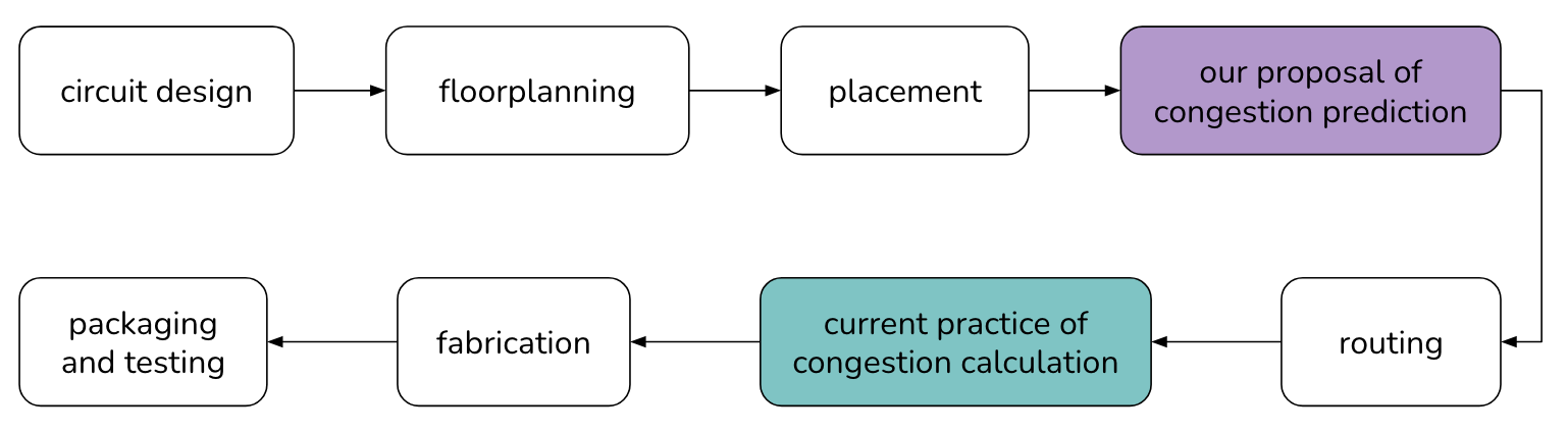VLSI Chip Design Flow

The chip’s functionality and logic are designed, which is then turned into a circuit representation. The components of this circuit are digitally placed onto the area of the chip, and then wires are digitally routed between them with computer programs, all before the chip is physically produced and tested. One of the issues that prevents chips from being produced is congestion, which is basically when there are too many wires in a certain area on a chip. However, to assess whether or not there is congestion in a chip, one has to go through both placement and routing, which are both timely and computationally expensive. To speed up this process, research has been done to predict congestion before routing and sometimes before placement. The approach we take aims to predict congestion post-placement pre-routing by turning a chip design into a graph and passing its structure and features through a graph neural network. Through our experiments, we hope to gain better insights about the strengths and shortcomings of graph neural network architectures, as well as insights about the data that can contribute to better congestion predictions.


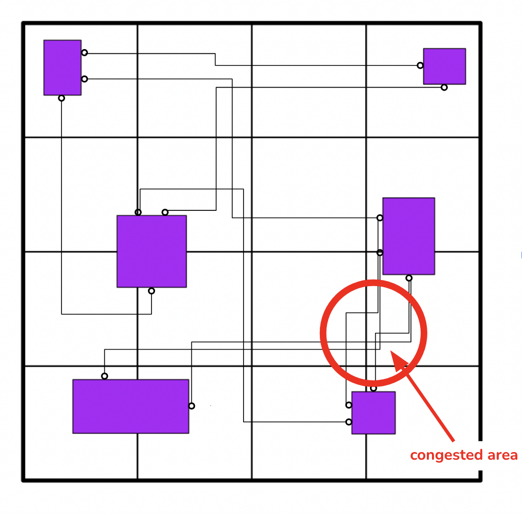
Congestion Depicted in a Netlist

Methods

The dataset we used was provided by Qualcomm and contained 13 different circuit designs, also known as netlists. Each of the netlists consisted of a few thousand instances, each of which one can think of as a node in the graph representation of the circuit. Each of those instances has a few given attributes, like name, the type of cell it is, and the x- and y-locations. These would serve as features to be passed into the graph neural network.

However, a graph neural network also needs to take in a representation of the connectivity of the graph. Because there are commonly more than two components in the circuit connected with a single wire, the connectivity provided to us was in an incidence matrix in the form of a hypergraph. An incidence matrix is a matrix where each row of the matrix represents a node in the graph, and each column represents an edge in the graph. If there is a connection between the node represented by row i and the edge represented by column j, there would be a 1 at (i, j) of the matrix, and a zero if there isn’t. A hypergraph is a graph where there are hyperedges, also known as nets, which are singular edges that connect multiple nodes. In our incidence matrix, the edges are hyperedges. We can multiple the incidence matrix by its transpose to find the adjacency matrix of the data, where now instead of rows representing nodes and columns representing edges, both rows and columns correspond to nodes, and there is a 1 at (i, j) if there is a connection between the two nodes. Taking the adjacency matrix and looking at the non-zero indices, we can construct an edge index. An edge index consists of two arrays that contain node indices. The node corresponding to the node index at position 0 in the first array is connected to the node corresponding to the node index at position 0 in the other array. This is the connectivity representation that we pass into our graph neural network.

We chose to use graph neural networks (GNNs) because the logic of a computer chip is encoded in its topology. We hoped that the information encoded in the topology will help the model capture things not captured by a purely visual approach like convolutional neural networks (CNNs), or traditional, tabular-based machine learning approaches. GNNs operate quite similarly to CNNs, except that the convolutions are performed over a node’s neighbors, as opposed to the convolutions being performed over a pixel’s neighbors, with information from each node’s neighbors being aggregated. Specifically, we use a type of GNN called the graph attention network (GAT) that uses an attention mechanism, which assigns a coefficient to each of the neighbors of each node. Higher coefficients are assigned to more important neighbors, and their information is weighed more heavily in the aggregation calculation. Intuitively, certain components in the chip design are more important to the chip’s function than others, and so the attention mechanism should be helpful.

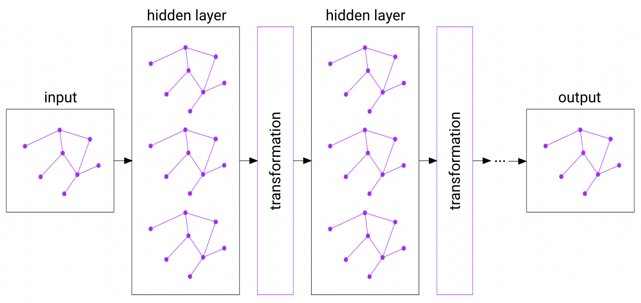Graph Neural Network

The choice of labels posed as an interesting challenge because of how the congestion data was given. The area of a chip is divided into a grid of roughly evenly sized rectangles. Each of these rectangles is called a Global Routing Cell, or GRC, and has a capacity value that describes the amount of wires that can be in the GRC. Alongside data on these capacity values, we are also given the demand values of each GRC that results from the routing process, which is simply the amount of wires that ended up being routed through the GRC. Congestion is formally defined as demand minus capacity, where values greater than zero indicate a congested GRC. The first decision we had to make was if we wanted to use congestion as the labels or demand as the labels. While congestion encodes information about capacity, we thought that that information was not necessary to include in the prediction. We thought it would be better if we only predicted the demand, then compared that demand to the given capacity at each of the GRCs. This brings us to our next challenge, which was that demand is given per GRC, not per instance. We could have directly predicted the demand of each GRC, but then we could not effectively make use of the connectivity data. We would have had to make each GRC into a supernode, making features based on the instances within the GRC and using information about the connections of the instances within the GRC to determine which other GRCs it is connected to. However, the reason we wanted to use GNNs in the first place is to capture the logic of the circuit encoded in its topology. Changing the connectivity information so that it is between GRCs instead of instances, we are no longer able to do that. So, we instead take the locations of each instance, make functions to locate the GRC they are located in, then assign the demand of that GRC to the instance. This is what we would use as the labels for our neural network.

We ran many different experiments, using different architectures, hyperparameters, and features. Due to complexities in passing in the connectivity data of multiple netlists, we only used one netlist for training and another for testing. It is worth noting the importance of normalizing the features in any model, as demand values typically range from around zero to fifty, and values like xloc, yloc, and height are given in tiny units that come in the tens of thousands. Conversely, it is important not to normalize the labels, as the small range of values will make it hard for the neural network to make accurate predictions when the differences between a demand of 28 and 29 gets shrunken down to a few tenths. In our experiments with architectures, we found that simply increasing the complexity of the model with more layers and hidden layers was not very effective. While in theory increased complexity should lead to easy overfitting of the training data, we repeatedly found that the GAT would predict the mean more and more commonly as we blindly increased model complexity. We realized that a relatively simple, 2 layer, 32 hidden layer, 8 head graph attention network with a linear layer performed best to overfit the training data. However, this model did not generalize well to test data, and we found that the distribution of the model’s predicted labels on the test data matched the distribution of the training data’s labels.

As a result, we looked to engineer features to improve our model performance, creating three features that we thought would be positively correlated with higher demand: GRC pin density, GRC cell density, and number of connections. GRC pin density is the total amount of pins in the GRC that the instance is in. Intuitively, we thought that the more pins there were in a GRC, the more wires would probably be there, which would mean higher demand. Similarly, GRC cell density is the total amount of cells in the GRC that the instance is in, and we thought that if there were more cells in the GRC, there would probably be more wires and higher demand. The number of connections is simply the number of wires that are connected to the instance, and we, again, thought that instances with more connections would probably mean overall higher demand in the GRC. Although information of the structure should be implicitly captured by the graph attention network, we thought explicitly defining the connections could help improve the model’s performance.

Results

Our GAT model with engineered features was our best model. In comparison to a basic XGBoost model and the GAT model without engineered features, the test MSE is higher. However, the distributions of those models’ predicted labels matches the distribution of the training data’s labels. If we look at the distribution of the GAT model with engineered features, however, we see that the shape of the distribution of predicted labels is similar to the shape fo the distribution of the test set’s labels, despite being centered differently. We believe that this indicates that this model is actually learning about the underlying patterns in the data, despite the overall MSE being higher. The predicted distribution is centered similarly to the center of the distribution of the training dataset, leading us to believe that if we were able to find a way to train on data from multiple netlists, we would be able to make a model that generalizes better. However, the ability of the GAT to learn underlying patterns in the data leads us to believe that a well-tuned model with engineered features could be incredibly effective at solving the congestion problem.


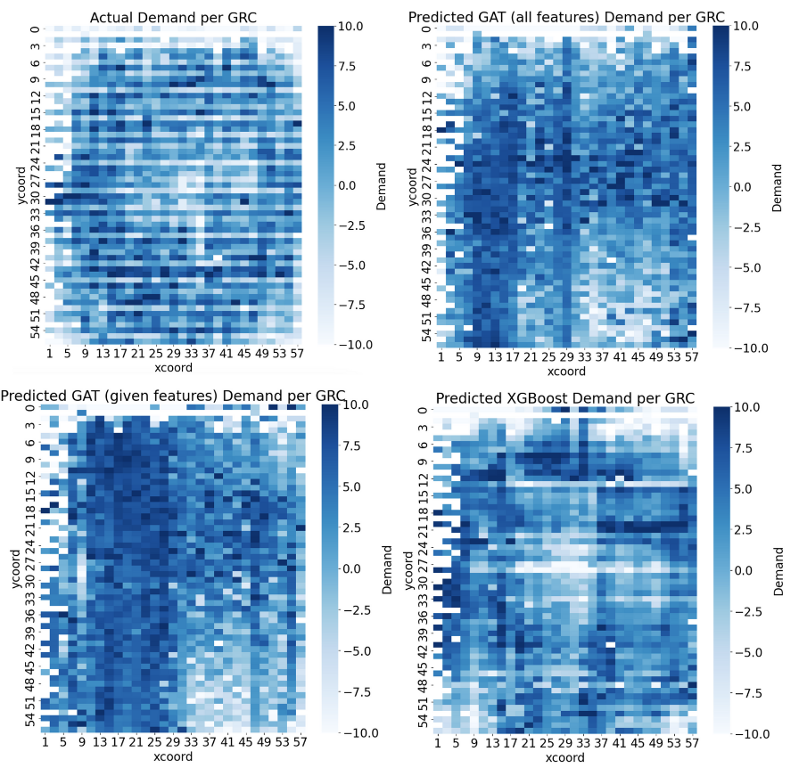
Our Results

Conclusion

The GAT appears to have great potential in solving the congestion problem. However, there is a lot of work to be done. Future work would start with finding a way to pass in connectivity data of multiple datasets, because that would allow us to train on multiple datasets and lead to better generalized results. After finding. Way to do that, we would then find ways to scale the architecture. We worked with relatively small netlists with thousands of instances, but netlists can have millions of nodes, and we would likely run into issues with memory and timing when trying to train models for this data. A more challenging final step after addressing these two issues would be predicting the demand in GRCs without instances. Right now, we use an instance-based prediction method where we predict the demand associated with the instance (assigned with the process described above), then average demand values over instances in a GRC to use as a predicted demand value for a GRC. Without instances, our model is not able to predict demand for a GRC if we approach it using this method. This is a pretty interesting challenge, and we would likely have to take a completely different approach from the instance-based prediction method that we are currently using if we want to address it properly. Until then, we plan on continuing work with instance-based methods, as graph neural networks appear to have promising results when applied in this way.

Index Terms

• Very Large-Scale Integration
• Routing Congestion
• Deep Learning
• Graph Attention Network
• Post-Placement
• Pre-Routing

Our project repository can be accessed at:
GitHub Repo